A Primer on Mathematical Modeling in the Study of Organisms and Their Parts
Systems Biology
How do mathematical models convey meaning? What is required to build a model? An introduction for biologists and philosophers.
Abstract
Mathematical modeling is a very powerful tool for understanding natural phenomena. Such a tool carries its own assumptions and should always be used critically. In this chapter, we highlight the key ingredients and steps of modeling and focus on their biological interpretation. In particular, we discuss the role of theoretical principles in writing models. We also highlight the meaning and interpretation of equations. The main aim of this chapter is to facilitate the interaction between biologists and mathematical modelers. We focus on the case of cell proliferation and motility in the context of multicellular organisms.
Keywords: Equations, Mathematical modeling, Parameters, Proliferation, Theory
A primer on mathematical modeling in the study of organisms and their parts
Abstract
Mathematical modeling is a very powerful tool to understand natural phenomena. Such a tool carries its own assumptions and should always be used critically. In this chapter we highlight the key ingredients and steps of modeling and focus on their biological interpretation. In particular, we discuss the role of theoretical principles in writing models. We also highlight the meaning and interpretation of equations. The main aim of this chapter is to facilitate the interaction between biologists and mathematical modelers. We focus on the case of cell proliferation and motility in the context of multicellular organisms.
Keywords : mathematical modeling, proliferation, theory, equations, parameters
1 Introduction
Mathematical modeling may serve many purposes such as performing quantitative predictions or making sense of a situation where reciprocal interactions are beyond informal analyses. For example, describing the properties of the diferent ionic channels of a neuron individually is not sufficient to understand how their combination entails the formation of action potentials. We need a mathematical analysis such as the one performed by the Hodgkin-Huxley model to gain such an understanding [1]. In this sense, mathematical modeling is required at some point in order to understand many biological phenomena. Let us emphasize that the perspective of modelers is usually different than the one of many experimentalists, especially in molecular biology. The latter field tends to emphasize the contribution of individual parts, but traditional reductionism [ 2] involves both the analysis of parts and the theoretical composition of parts to understand the whole, usually by means of mathematical analysis. Without the latter move, it is never clear whether the parts analyzed individually are sufficient to explain how the phenomenon under study comes to be or whether key processes are missing.
We want to emphasize the difference between mathematical models on the one side and theories on the other side. Of course modelization belongs to the broad category of theoretical work by contrast with experimental work. However, in this text, we will refer to theory in the precise sense of a broad conceptual framework such as evolutionary theory. Evolutionary theory has been initially formulated without explicit mathematics. Evolutionary theory has actually led to different categories of mathematical analyses such as population genetics or phyllogenetic analysis which are very different mathematically. Theoretical frameworks typically guide modelization and contributes to justify mathematical models.
Mathematical modeling raises several difficulties in the study of organisms.
The first one is that most biologists do not have the mathematical or physical background to assess the meaning and the validity of models. The division of labor in interdisciplinary projects is an efficient way to work but it should at least be completed by an understanding of the principles at play in every part of the work. Otherwise, the coherence of the knowledge that result from this work is not ensured.
The second difficulty is intrinsic. Living objects have theoretical specificities that make mathematical modeling difficult or at least limit its meaning. These specificities are at least of two kinds.
- Current organisms are the result of an evolutive and developmental history which means that many contingent events are deeply inscribed in the organization of living being. By contrast the aim of mathematical modeling is usually to make explicit the necessity of an outcome. For more on this issue, see [3].
- The study of a part X of an organism is not completely meaningful by itself. Instead, the inscription of this part inside the organism and in particular the role that this part plays is a mandatory object of study to assess the biological relevance of the properties of X that are under study. As such, the modelization of X per se is insufficient and requires a supplementary discussion [4].
The third difficulty is that there are no well established theoretical principles to frame model writing in physiology or developmental biology [5]. In particular, cells are elementary objects since the cell theory states that there is no living things without cells. However, cells have complex organizations themselves. Modeling their behavior (note 1) is therefore challenging and requires appropriate theoretical assumptions to ensure that this modeling has a robust biological meaning.
A theoretical way to organize the mathematical modeling of cell behaviors is to propose a default state, that is to say to make explicit a state of reference that takes place without the need of particular constraints, input or signal. We think that proliferation with variation and motility should be used as a default state [6, 7]. Under this assumption, cells spontaneously proliferate. By contrast, quiescence should be explained by constraints explicitly limiting or even preventing cell proliferation. The same reasoning applies mutadis mutandis to motility. This assumption has been used to model mammary gland morphogenesis and helps to systematize the mathematical analysis of cellular populations [8].
In this chapter we will focus on model writing. Our aim is not to emphasize the technical aspects of mathematical analysis. Instead, this text aims to help biologists to understand modelization in order to better interact with modelers. Reciprocally, we also highlight theoretical specificities of biology which may be of help to modelers. Of course, the usual way to divide chapters in this book series is not entirely appropriate for the topic of our chapter. We still kept this structure and follow it in a metaphorical sense. In materials, we are describing key conceptual and mathematical ingredients of models. In methods, we will focus on the writing and analysis of models per se.
2 Materials
2.1 Parameters and states
2.1.1 Parameters
Parameters are quantities that play a role in the system but which are not significantly impacted by the system’s behavior at the time scale of the phenomenon under study. From an experimentalist’s point of view, there are two kinds of parameters. Some parameters correspond to a quantity that is explicitly set by the experimenter such as the temperature, the size of a plate or the concentration of a relevant compound in the media. Other parameters correspond to properties of parts under study, such as the speed of a chemical reaction, the elasticity of collagen or the division rate
Identifying relevant parameters has actually two different meaning :
- Parameters that will be used explicitly in the model are parameters whose value is required to deduce the behavior of the system. The dynamics of the system depends explicitly on the value of these parameters. A fortiori, parameters that correspond to different treatments leading to a response will fall under this category. Note that the importance of some parameters usually appear in other steps of modeling.
- Theoretical parameters correspond to parameters that we know are relevant and even mandatory for the process to take place but that we can keep implicit in our model. For example, the concentration of oxygen in the media is usually not made explicit in a model of an in vitro experiment even though it is relevant for the very survival of the cells studied. Of course, there is usually a cornucopia of this sort of parameters, for example the many components of the serum.
2.1.2 State space
The state of an object describes its situation at a given time. The state is composed of one or several quantities, see note 3. By contrast with parameters, the notion of state is restricted to those aspects of the system which will change as a result of explicit causes or randomness intrinsic to the system described. The usual approach, inherited from physics, is to propose a set of possible states that does not change during the dynamics. Then the changes of the system will be changes of states while staying among these possible states. For example, we can describe a cell population in a very simple manner by the number of cells n(t). Then, the state space is all the possible values for n, that is to say the positive integers.
Usually, the changes of state depend on the state of the system which means that the state has a causal power, which can be either direct or indirect. A direct causal power is illustrated by n which is the number of cells that are actively proliferating in the example above and thus trigger the changes in n. An indirect causal power corresponds, for example, to the position of a cell provided that some positions are too crowded for cells to proliferate.
2.1.3 Parameter versus state
Deciding whether a given quantity should be described as a parameter or as an element of the state space is a theoretical decision that is sometimes difficult, see also note 4. The heart of the matter is to analyze the role of this quantity but it also depends on the modeling aims.
- Does this quantity change in a quantitatively significant way at the time scale of the phenomenon of interest ? If no it should be a parameter. If yes :
- Are the changes of this quantity required to observe the phenomenon one wants to explain ? If yes, it should be a part of the state space. If no :
- Do we want to perform precise quantitative predictions ? If yes, then the quantity should be a part of the state space and a parameter otherwise.
In the following, we will call “description space” the combination of the state space and parameters.
2.2 Equations
Equations are often seen as intimidating by experimental biologists. Our aim here and in the following subsection is to help demystify them. In the modeling process, equations are the final explicitation of how changes occur and causes act in a model. As a result understanding them is of paramount importance to understand the assumptions of a model.
The basic rule of modeling is extremely simple. Parameters do not require equations since they are set externally. However, the value of states are unspecified. As a result, equations are required to describe how states change. More precisely, modelers require an equation for each quantity describing the state. Quantities of the state space are degrees of freedom, and these degrees of freedom have to be “removed” by equations for the model to perform predictions. These equations need to be independent in the sense that they need to capture different aspects of the system : copying twice the same equation obviously does not constrain the states. Equations typically come in two kinds :
- Equations that relate different quantities of the state space. For example, if we have n the total number of cells and two possible cell types with cell counts n1 and n2, then we will always have
- Equations that describe a change of state as a function of the state. These equations typically take two different forms, depending on the representation of time which may be either continuous or discrete, see note 5. In continuous time, modelers use differential equations, for example
2.3 Invariants and symmetries
We have discussed the role of equations, now let us expand on their structure. Let us start with the equation mentioned above :
Alternatively, this equation is equivalent to
Probabilities may also be analyzed on the basis of symmetries. Randomness may be defined as unpredictability in a given theoretical frame and is more general than probabilities. To define probabilities, two steps have to be performed. The modeler needs to define a space of possibilities and then to define the probabilities of these possibilities. The most meaningful way to do the latter is to figure out possibilities that are equivalent, that is to say symmetric. For example, in a homogeneous environment, all directions are equivalent and thus would be assigned the same probabilities. A cell, in this situation, would have the same chance to choose any of these directions assuming that the cell’s organization is not already oriented in space, see also note 6. In physics, a common assumption is to consider that states which have the same energy have the same probabilities.
Now there are several ways to write equations, independently of their deterministic or stochastic nature :
- Symmetry based writing is exemplified by the model of exponential growth above. In this case, the equation has a genuine meaning. Of course the model conveys approximations which are not always valid, but the terms of the equation are biologically meaningful. This also ensure that all mathematical outputs of the model may be interpreted biologically.
- Equations may also be based on a mathematical reasoning which provides a legitimacy to their form but restricts their biological interpretations. For example, many mathematical functions may be approximated around 0 by the sum
where k is the maximum of the population. Le us remark that we have written the equation in two different forms, we come back on this in note 7. The solution of this equation is the classical logistic function.
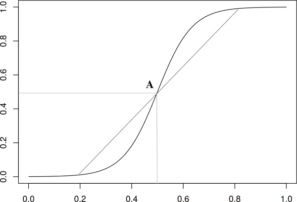
Note however that this equation has symmetries which are dubious from a biological viewpoint : the way the population takes off is identical to the way it saturates because the logistic equation has a center of symmetry, A in figure, see also [11].
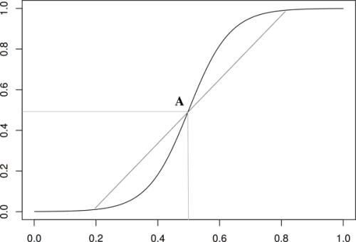
Figure 1 : The logistic function. This function is often used to model a growth with constraints leading to a saturation. However, this function possess a center of symmetry, A, which implies that the initial exponential growth is exactly equivalent to the way the growth saturates. This is biologically problematic : there is an initial lag phase and the saturation trigger causes that are not significant in the initial growth leading for example to cell death [12]. - The last way to write equations is called heuristic. The idea is to use functions that mimic quantitatively and to some extent qualitatively the phenomenon under study. Of course this method is less meaningful that the others but it is often required when the knowledge of the underlying phenomenon is not sufficient.
2.4 Theoretical principles
Theoretical principles are powerful tools to write equations that convey biological meaning. Let us provide a few examples.
- Cell theory implies that cells come from the proliferation of other cells and excludes spontaneous generation.
- Classical mechanics aims to understand movements in space. The acceleration of an object requires that a mechanical force is exerted on this object. Note that the principle of reaction states that if A exerts a force on B, then B exerts the same force with opposite direction on A. Therefore, there is an equivalence between “A exerts a force” and “a force is exerted on A” from the point of view of classical mechanics. The difficulty lies in the forces exerted by cells as cells can consume free energy to exert many kinds of forces. Cells are neither an elastic nor a bag of water, they possess agency which leads us to the next point.
- As explained in introduction, the reference to a default state helps to write equations that pertain to cellular behaviors. There are many aspects that contribute to cellular proliferation and motility. The writing of an equation such as the logistic model is not about all these factors and should not be interpreted as such. Instead, it assumes proliferation on the one side and one or several factors that constrain proliferation on the other side.
3 Methods
3.1 Model writing
Model writing may have different levels of precision and ambition. Models can be a proof of concept, that is to say the genuine proof that some hypotheses explain a given behavior or even proofs of the theoretical possibility of a behavior. Proof of concept do not include a complete proof that the natural phenomenon genuinely behave like the model. On the opposite end of the spectrum, models may aim at quantitative predictions. Usually, it is good practice to start from a crude model and after that to go for more detailed and quantitative analyses depending on the experimental possibilities.
We will now provide a short walkthrough for writing an initial model :
- Specify the aims of the model. Models cannot answer all questions at once, and it is crucial to be clear on the aim of a model before attempting to write it. Of course, these aims may be adjusted afterwards. The scope of the model should also depend on the experimental methods that link it to reality.
- Analyze the level of description that is mandatory for the model to explain the target phenomenon. Usually, the simplest the description is the better. When cells do not constrain each other, describing cells by their count n is sufficient. By contrast, if cells constrain each other, for example if they are in organized 3d structures it can be necessary to take into account the position of each individual cell which leads to a list of positions
- List the theoretical principles that are relevant to the phenomenon. These principles can be properly biological and pertain to cell theory, the notion of default state, biological organization or evolution. Physico-chemical principles may also be useful such as mechanics or the balance of chemical reactions.
- List the relevant states and parameters. These quantities are the ones that are expected to play a causal role that pertains to the aim of the model. This list will probably not be definitive, and will be adjusted in further steps. In all cases, we cannot emphasize enough that aiming for exhaustivity is the modeler’s worst enemy. Biologists need to take many factors into account when designing an experimental protocol, it is a mistake to try to model all of these factors.
- The crucial step is to propose mathematical relations between states and their changes. We have described in sections 2.2 and 2.3 what kinds of relation can be used. Usually these relations will involve supplementary parameters whose relevance was not obvious initially. Let us emphasize here that the key to robust models is to base it on sufficiently solid grounds. A model where all relations are heuristic will probably not be robust. As such, figuring out the robust and meaningful relations that can be used is crucial.
- The last step is to analyze the consequences of the model. We describe this step with more details below. What matters here is that the models may work as intended, in which case it may be refined by adding further details. The model may also lead to unrealistic consequences and not lead to the expected results. In these latter cases, the issue may lie in the formulation of the relations above, in the choice of the variables or in oversimplifications. In all cases the model requires a revision.
Writing a model is similar to the chess game in that the anticipation of all these steps from the beginning helps. The steps that we have described are all required but a central aspect of modeling is to gain a precise intuition of what determines the system’s behavior. Once this intuition is gained, it guides the specification of the model at all step. Reciprocally, these steps help to gain such an intuition.
3.2 Model analysis
In this section, we will not cover all the main ways to analyze model since this subject is far too vast and depends on the mathematical structures used in the models. Instead, we will focus on the outcome of model analyses.
3.2.1 Analytic methods
Analytic methods consist in the mathematical analysis of a model. They should always be preferred to simulations when the model is tractable, even at the cost of using simplifying hypotheses.
- Asymptotic reasoning is a fundamental method to study models. The underlying idea is that models are always a bit complicated. To make sense of them, we can look at the dynamics after enough time which simplifies the outcome. For example, the outcome of the logistic function discussed above will always be an equilibrium point, where the population is at a maximum. Mathematically, “enough” time means infinite time, hence the term asymptotic. In practice “infinite” means “large in comparison with the characteristic times of the dynamics”, which may not be long from a human point of view. For example, a typical culture of bacteria reaches a maximum after less than day. Asymptotic behaviors may be more complicated such as oscillations or strange attractors.
- Steady states analysis. In fairly complex situations, for example when both space and time are involved, a usual approach is to analyze states that are sustained over time. For example, in the analysis of epithelial morphogenesis, it is possible to consider how the shape of a duct is sustained over time.
- Stability analysis. A very common analytic method is to find equibria, that is to say situations where the changes stop (dx/dt=0 for all state variable x). For example,
Near 0,
Near k, let us write
In this case, the small variation
- Special cases. In some situations, qualitatively remarkable behaviors appear for specific values of the parameters. Studying these cases is interesting per se, even though the odds for parameters to have specific value are slim without an explicit reason for this paramter to be set at this value. However, in biology the value of some parameters are the result of biological evolution and specific value can become relevant when the associated qualitative behavior is biologically meaningful [13,14].
- Parameter rewriting. One of the major practical advantages of analytical methods is to prove the relevance of parameters that are key to understand the behavior of a system. These “new” parameters are usually combinations of the initial parameters. We have implicitly done this operation in section 2.3. Instead of writing
3.2.2 Numerical methods – simulations
Simulations have a major strength and a major weakness. Their strength lies in their ability to handle complicated situations that are not tractable analytically. Their weakness is that each simulation run provides a particular trajectory which cannot a priori be assumed to be representative of the dynamical possibilities of the model.
In this sense, the outcome of simulations may be compared to empirical results, except that simulation are transparent : it is possible to track all variables of interest over time. Of course, the outcome of simulations is artificial and only as good as the initial model.
Last, there is almost always a loss when going from a mathematical model to a computer simulation. Computer simulation are always about discrete objects and deterministic functions. Randomness and continua are always approximated in simulations and mathematical care is required to ensure that the qualitative features of simulations are feature of the mathematical model and not artifacts of the transposition of the model into a computer program. A subfield of mathematics, numerical analysis, is devoted to this issue.
3.2.3 Results
We want to emphasize two points to conclude this section.
First, it is not sufficient for a model to provide the qualitative or even quantitative behavior expected for this model to be correct. The validation of a model is based on the validation of a process and of the way this process takes place. As a result, it is necessary to explore the predictions of the model to verify them experimentally. All outcomes that we have described in 3.2.1 may be used to do so on top of a direct verification of the assumptions of the model themselves. Of course, it is never possible to verify everything experimentally, therefore the focus should be on aspects that are unlikely except in the light of the model.
Second, modeling focuses on a specific part and a specific process. However, this part and this process take place in an organism. Their physiological meaning, or possible lack thereof, should be analyzed. We are developing a framework to perform this kind of analysis [15,4] but it can also be performed informally by looking at the consequences of the part considered for the rest of the organism.
4 Notes
- In biology, behavior usually has an ethological meaning and evolution refers to the theory evolution. In the mathematical context, these words have a broader meaning. They both typically refer to the properties of dynamics. For example, the behavior of a population without constrain is exponential growth.
- Parameters that play a role in an equation are defined in two different ways. They are defined by their role in the equation and by their biological interpretation. For example, the division rate
- A state may be composed of several quantities, let’s say k, n, m. It is possible to write the state by the three quantities independently or to join them in one vector X=(k,n,m). The two viewpoints are of course equivalent but they lead to different mathematical methods and ways to see the problem. The second viewpoint shows that it is always valid to consider that the state is a single mathematical object and not just a plurality of quantities.
- The notion of organization in the sense of a specific interdependence between parts [4] implies that most parameters are a consequence of others parts, at other time scales. As a result, modeling a given quantity as a parameter is only valid for some time scales, and is acceptable when these time scales are the ones at which the process modeled takes place.
- The choice between a model based on discrete or on continuous time is base on several criteria. For example, if the proliferation of cells is synchronized, there is a discrete nature of the phenomenon that strongly suggests to represent the dynamics in discrete time. In this case the discrete time corresponds to an objective aspect of the phenomenon. On the opposite, when cells divide at all times in the population, a representation in continuous time is more adequate. In order to perform simulations, time may still be discretized but the status of the discrete structure is then different than in the first case : discretization is then arbitrary and serves the purpose of approximating the continuum. To distinguish the two situations, a simple question should be asked. What is the meaning of the time difference between two time points. In the first case, this time difference has a biological meaning, in the second it is arbitrary and just small enough for the approximation to be acceptable.
- Probabilities over continuous possibilities are somewhat subtle. Let us show why : let us say that all directions are equivalent, thus all angles in the interval [0,360[ are equivalent. They are equivalent, so their probabilities are all the same value p. However, there is an infinite number of possible angles, so the sum of all the probabilities of all possibilities would be infinite. Over the continuum, probabilities are assigned to sets and in particular to intervals, not individual possibilities.
- There are many equivalent ways to write a mathematical term. The choice of a specific way to write a term conveys meaning and corresponds to an interpretation of this term. For example, in the text, we transformed
- The number of quantities that form the state space is called its dimension. The dimension of the phase space is a crucial matter for its mathematical analysis. Basically, low dimensions such as 3 or below are more tractable and easier to represent. High dimensions may also be tractable if many dimensions play equivalent roles (even in infinite dimension). A large number of heterogeneous quantities (10 or 20) is complicated to analyze even with computer simulations because this situation is associated with many possibilities for the initial conditions and for the parameters making it difficult to “probe” the different qualitative possibilities of the model.
- It is very common in modeling to use the words “small” and “large”. A small (resp. large) quantity is a quantity that is assumed to be small (resp. large) enough so that a given approximation can be performed. For example, a large time in the context of the logistic equation means that the population is approximately at the maximum k. Similarly, infinite and large are very close notions in most practical cases. For example, a very large capacity k leads to
References
- Beeman, D. (2013). Hodgkin-Huxley Model, pages 1–13. Encyclopedia of Computational Neuroscience. Springer New York, New York, NY. Doi : 10.1007/978-1-4614-7320-6_127-3
- Descartes, R. (2016). Discours de la méthode. Flammarion.
- Montévil, M., Mossio, M., Pocheville, A., and Longo, G. (2016a). Theoretical principles for biology : Variation. Progress in Biophysics and Molecular Biology, 122(1) : 36 – 50. Doi : 10.1016/j.pbiomolbio.2016.08.005
- Mossio, M., Montévil, M., and Longo, G. (2016). Theoretical principles for biology : Organization. Progress in Biophysics and Molecular Biology, 122(1) : 24 – 35. Doi : 10.1016/j.pbiomolbio.2016.07.005
- Noble, D. (2010). Biophysics and systems biology. Philosophical Transactions of the Royal Society A : Mathematical, Physical and Engineering Sciences, 368(1914) : 1125. Doi : 10.1098/rsta.2009.0245
- Sonnenschein, C. and Soto, A. (1999). The society of cells : cancer and control of cell proliferation. Springer Verlag, New York.
- Soto, A. M., Longo, G., Montévil, M., and Sonnenschein, C. (2016). The biological default state of cell proliferation with variation and motility, a fundamental principle for a theory of organisms. Progress in Biophysics and Molecular Biology, 122(1) : 16 – 23. Doi : 10.1016/j.pbiomolbio.2016.06.006
- Montévil, M., Speroni, L., Sonnenschein, C., and Soto, A. M. (2016b). Modeling mammary organogenesis from biological first principles : Cells and their physical constraints. Progress in Biophysics and Molecular Biology, 122(1) : 58 – 69. Doi : 10.1016/j.pbiomolbio.2016.08.004
- D’Anselmi, F., Valerio, M., Cucina, A., Galli, L., Proietti, S., Dinicola, S., Pasqualato, A., Manetti, C., Ricci, G., Giuliani, A., and Bizzarri, M. (2011). Metabolism and cell shape in cancer : A fractal analysis. The International Journal of Biochemistry & Cell Biology, 43(7) : 1052 – 1058. Metabolic Pathways in Cancer. Doi : 10.1016/j.biocel.2010.05.002
- Longo, G. and Montévil, M. (2014). Perspectives on Organisms : Biological time, symmetries and singularities. Lecture Notes in Morphogenesis. Springer, Dordrecht. Doi : 10.1007/978-3-642-35938-5
- Tjørve, E. (2003). Shapes and functions of species–area curves : a review of possible models. Journal of Biogeography, 30(6) : 827 – 835. Doi : 10.1046/j.1365-2699.2003.00877.x
- Hoehler, T. M. and Jorgensen, B. B. (2013). Microbial life under extreme energy limitation. Nat Rev Micro, 11(2) : 83 – 94. Doi : 10.1038/nrmicro2939
- Camalet, S., Duke, T., Julicher, F., and Prost, J. (2000). Auditory sensitivity provided by self-tuned critical oscillations of hair cells. Proceedings of the National Academy of Sciences, pages 3183 – 3188. Doi : 10.1073/pnas.97.7.3183
- Lesne, A. and Victor, J.-M. (2006). Chromatin fiber functional organization : Some plausible models. Eur Phys J E Soft Matter, 19(3) : 279 – 290. Doi : 10.1140/epje/i2005-10050-6
- Montévil, M. and Mossio, M. (2015). Biological organisation as closure of constraints. Journal of Theoretical Biology, 372(0) : 179 – 191. Doi : 10.1016/j.jtbi.2015.02.029
∗ Montévil M. (2018) A Primer on Mathematical Modeling in the Study of Organisms and Their Parts. In: Bizzarri M. (eds) Systems Biology. Methods in Molecular Biology, vol 1702. Humana Press, New York, NY. Doi : 10.1007/978-1-4939-7456-6_4
† Laboratoire "Matière et Systèmes Complexes" (MSC), UMR 7057 CNRS, Université Paris 7 Diderot, 75205 Paris Cedex 13, France and Institut d’Histoire et de Philosophie des Sciences et des Techniques (IHPST) - UMR 8590 Paris, France.